Building an image classifier using convolutional neural networks
- asa5604
- Mar 26, 2023
- 8 min read
Updated: Mar 26, 2023
A key means of expressing emotions is through facial expressions. We are now able to create systems that can recognize facial emotions automatically thanks to the development of machine learning and computer vision. Our objective in this research is to create an image classifier that can precisely identify face expressions in photographs.
We will use the Facial Expression dataset available on Kaggle, which contains 35,887 grayscale images of faces, each labeled with one of seven emotions: angry, disgust, fear, happy, neutral, sad, and surprise. Our goal is to develop a deep learning model that can correctly categorize these photographs into the many emotions they represent.
Beginning with Google Colab
Google Colab will serve as our primary computing platform. With access to sophisticated hardware like GPUs and TPUs, Colab is a free cloud-based platform that enables us to run Python code in a Jupyter notebook environment.
Here's a link to my Colab Notebook
Here's a link to my Github repo
Essential imports
Also import tensorflow as tf
Getting the Data Ready
Preprocessing the data is necessary before our image classifier can be trained. In order to do this, the images must first be loaded into memory before being fixed in size and having their pixel values normalized.
We'll load the photos and run the preprocessing using the Keras ImageDataGenerator class. We may load images in batches using the ImageDataGenerator class, which is helpful for deep learning model training.
Here's the link to the Dataset
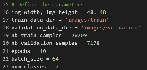
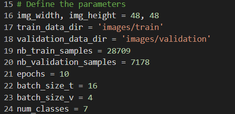
This code defines various parameters that will be used in the training of the image classifier model.
img_width and img_height represent the size of the images that will be used as input to the model.
train_data_dir and validation_data_dir specify the directories containing the training and validation data, respectively.
nb_train_samples and nb_validation_samples represent the number of training and validation samples, respectively.
epochs specifies the number of times the model will iterate over the entire training dataset.
batch_size is the number of samples that will be fed to the model at once during training.
num_classes specifies the number of classes (i.e., emotions) that the model will be trained to classify[5].
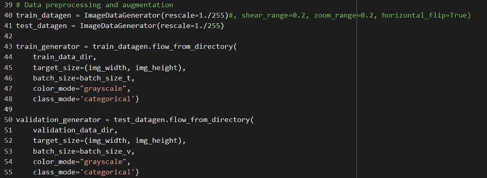
The training set's augmented data is produced using the ImageDataGenerator class. For the network to learn properly in this instance, we simply use rescale, which reduces the pixel values to a range between 0 and 1. Although they might also be employed, other augmentation methods like rotation, zooming, and flipping are not in this example.
Data is loaded from directories in batches using the flow_from_directory method. It accepts as parameters the directory path, batch size, color mode, class mode, and picture target size. Since the photos are grayscale in this instance, color_mode="grayscale" is applied. We have numerous classes for classification, thus the class_mode is set to "categorical".[5]
Building the Model(S)
Now that we have prepared the data, we can start building the deep learning model. We will use a convolutional neural network (CNN) for this task, which is a type of neural network that is particularly suited for image classification tasks.
MODEL 1

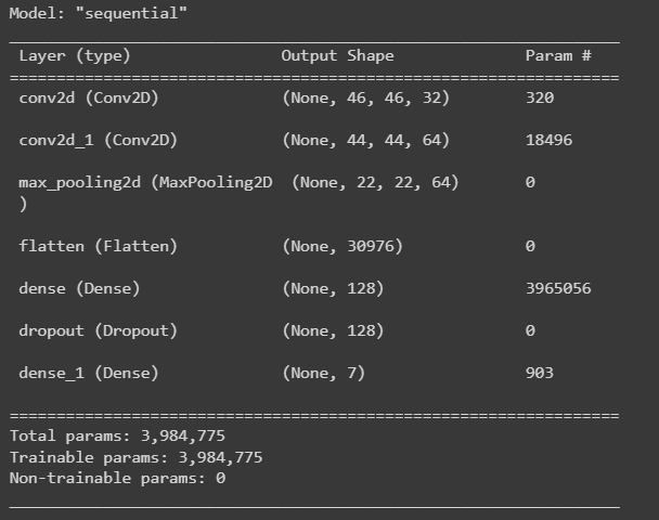
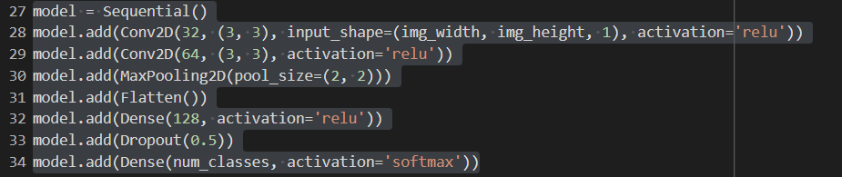
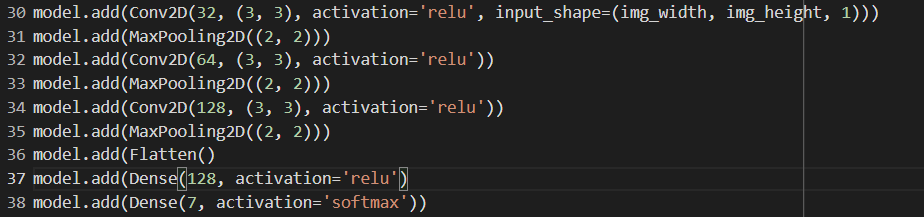
A straightforward convolutional neural network (CNN) model for image categorization is defined by this code. [1]Below is a description of each layer:
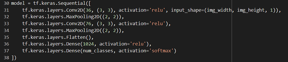
Conv2D(32, (3, 3), input_shape = (img_width, img_height, 1), activation = "relu" It accepts an input picture with the following dimensions: (img_width, img_height, 1), where the last dimension is the number of channels. This is the first convolutional layer with 32 filters of size 3x3. (1 for grayscale, 3 for RGB). ReLU, which is frequently employed in CNNs to introduce nonlinearity, is the activation function used.
Conv2D(64, (3, 3), activation='relu'): This convolutional layer has 64 3x3 filters in its second convolutional layer. The ReLU activation function is applied to the output of the first convolutional layer.
A max pooling layer with a pool size of 2x2 that reduces the output's spatial dimensions by a factor of 2 is called MaxPooling2D(pool_size=(2, 2)). By doing so, overfitting is avoided and the number of parameters is reduced.
The output of the preceding layer is flattened by the flatten() layer into a 1D vector, which can subsequently be fed into a dense layer.
Dense(128, activation="relu"): This dense layer has 128 neurons and the ReLU activation function. It is fully linked. It accepts as input the previous layer's output that has been flattened.
Dropout(0.5): During training, a dropout layer with a dropout rate of 0.5 randomly removes half of the neurons from the layer above. This lessens the chance of overfitting.
Dense(num_classes, activation='softmax'): This is the last output layer used for multi-class classification, with num_classes neurons and the softmax activation function. The projected class probabilities for the input image are represented in this layer's output[1].
This CNN model's overall architecture is ideal for small to medium-sized picture classification problems because it is reasonably straightforward. However, more intricate and deeper architectures can be required to obtain more accuracy depending on the difficulty of the task and the amount of the dataset.
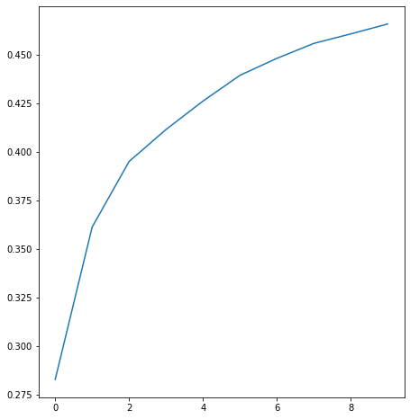
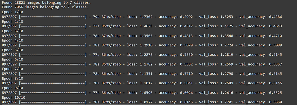
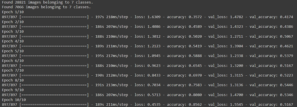
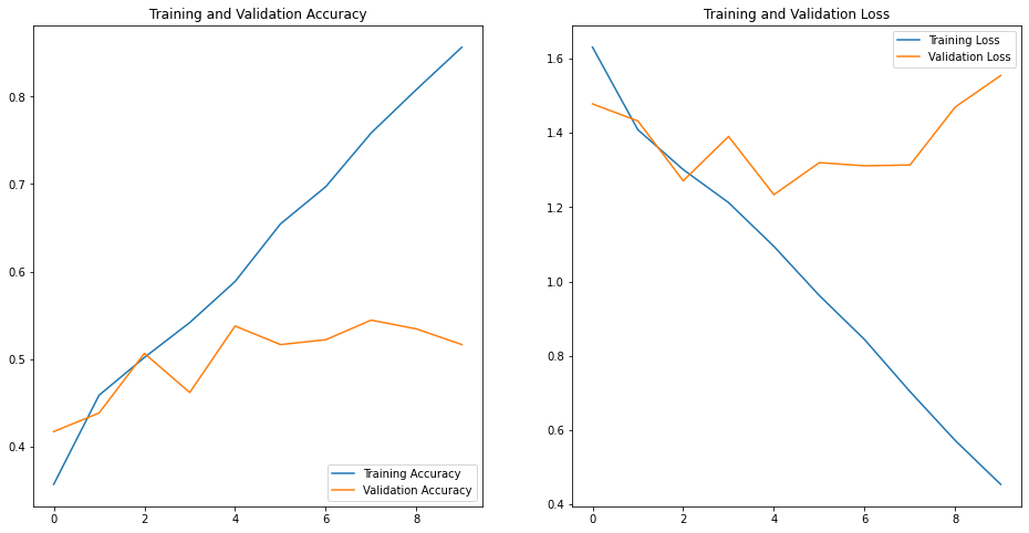
Model 1 Results:-
Train acc = 46
Valid acc = 39

As you can see from the above result this is a very inefficient and non optimal classifier due to :
1) As seen from fig-1 no. of validation samples are less compared to the training samples
and I have used the same batch size for both of them, this is the first cause of inaccuracy which will be improved in the further models
2) Also the conv2D layers does not have a soft max function. Without the softmax activation function, the outputs of the final Dense layer would be unnormalized and could not be interpreted as class probabilities. Therefore, softmax is important in this context to obtain meaningful predictions for multi-class image classification.
Model 1 Visuals:-
CONTRIBUTIONS & IMPROVEMENTS IN MODEL-1
MODEL 2
UPGRADES FROM MODEL-1
Model 2 Results:-
Train acc = 59
Valid acc = 51

As you can see from the above result this is still a very inefficient and non optimal classifier due to :
2) less complex neurons[2] and layers, now we will inculde more layers and try to make the model slightly complex
Model 2 Visuals:-
MODEL 3
UPGRADES FROM MODEL-1,2
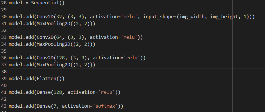
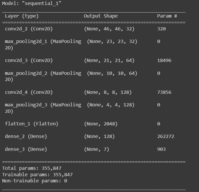
This model's architecture is made up of a number of convolutional layers, pooling layers, and two thick layers at the end. A grayscale image with the dimensions (img_width, img_height, 1) serves as the model's input. Here is a quick summary of each layer:
Conv2D layer with a ReLU activation function, 32 filters, and a (3, 3) filter size. By combining the input image with a number of filters to create a set of activation maps, this layer conducts feature extraction.
a pool size of in the MaxPooling2D layer (2, 2). The activation maps created by the preceding layer are downsampled in this layer, which reduces the output's spatial dimensions.
A second Conv2D layer with a ReLU activation function, 64 filters, and a (3, 3) filter size. This additional layer[3]
Using the pool size of another MaxPooling2D layer, (2, 2).
A third Conv2D layer with a ReLU activation function, 128 filters, and a (3, 3) filter size. This layer keeps on extracting more intricate features from the output of the layer before it.
Using the pool size of another MaxPooling2D layer, (2, 2).
Using a flatten layer, the output from the preceding layer is converted into a 1D vector that may be fed into a dense layer [3].
a dense layer with a ReLU activation function and 128 neurons. The characteristics retrieved by the previous convolutional layer are combined in this layer to achieve high-level feature extraction.
If this is a multi-class classification problem, there is another dense layer with 7 neurons and a softmax activation function. The final output from this layer displays the assumed class probabilities for the input image[3].
Overall, this model architecture offers a straightforward but efficient method for jobs involving image classification. But by adjusting the hyperparameters, adding more layers or filters, and adding other methods like regularization or data augmentation, the model's performance can be enhanced[5].
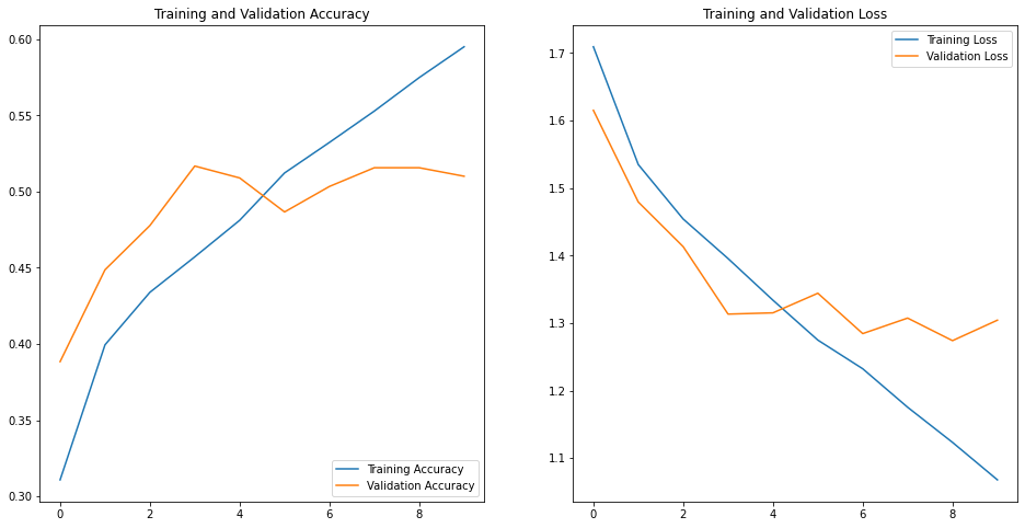
Model 3 Results:-
Train acc = 61
Valid acc = 55
As you can see from the above result this is a very inefficient and non optimal classifier due to :
Model 3 Visuals:-

MODEL 4
UPGRADES FROM MODEL-1,2,3
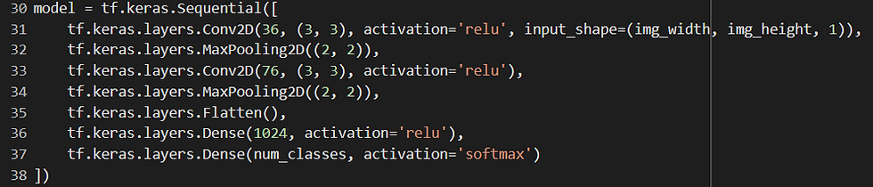
Following the 36-76-1024 approach
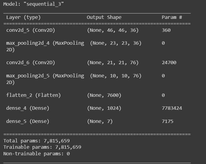
Conv2D layer with'relu' activation function and 36 filters of size (3, 3). According to the input shape of (img_width, img_height, 1), the input is a grayscale image with dimensions of img_width and img_height.
MaxPooling2D layer with pool size (2, 2), which shrinks the output feature maps' spatial extent.
Conv2D layer with'relu' activation function and 76 filters of size 3 and 3.
the pool size-specific MaxPooling2D layer (2, 2).
The flatten layer converts the output of the layer before into a 1D array.
dense layer with activation function "relu" and 1024 units[4].
Dense layer with the activation function "softmax" and the number of classes (num_classes units) that we wish to classify the images into. The outputs are normalized using the "softmax" function to total to 1, making them comprehensible as probabilities[4].
Convolutional layers, which extract picture features, are combined with dense layers in this model to carry out the actual classification based on those characteristics. To maximize the model's performance for a particular task, the activation functions, number of filters, and number of units in the dense layers can all be adjusted.
Overall, this model architecture offers a slightly efficient method for jobs involving image classification as compared to the previous models.
Model 4 Results:-
Train acc = 85
Valid acc = 51
As you can see from the above results this model's training accuracy is far better than the previous models but the validation accuracy decreased slightly as compared to model 3.
Also this model is facing slight issues of overfitting
Model 4 Visuals:-
MODELS COMPARISON
it sets the size of the figure and the width of the bars. It creates the bar chart for train accuracies using the plt.bar() function, and then creates the bar chart for validation accuracies with the same function, but with a slight shift in the x-axis position using x_pos + bar_width.
VISUALS

Overall Contributions
Used different batch sizes for training and validation sets as
# of validation sets< # of training sets(model 2)
Used a slightly different architecture(hyperparameter tuning)in model 3 as compared to model 2
The 2nd model has two convolutional layers with 32 and 64 filters respectively, followed by max pooling, flattening, a dense layer with 128 neurons, dropout, and a dense layer with the number of output classes using softmax activation.
The 3rd model has three convolutional layers with 32, 64, and 128 filters respectively, followed by max pooling, flattening, a dense layer with 128 neurons, and a dense layer with the number of output classes using softmax activation.
In other words, the 3rd model has more convolutional filters and layers, but does not have dropout regularization. The 2nd model may perform better when there is limited data or when regularization is needed, while the 3rd model may perform better with more data and a more complex problem.
Tweaked the model 3 and made a model 4 with the following contributions:
Model 3 has 3 convolutional layers with max-pooling layers in between, followed by a flatten layer, a dense layer with 128 neurons, and a softmax output layer with 7 neurons. Model 4 also has convolutional layers with max-pooling layers, followed by a flatten layer, a dense layer with 1024 neurons, and a softmax output layer with 7 neurons. The main difference between the two models is the number of convolutional layers and the number of neurons in the dense layer. Model 4 has more convolutional layers and a denser layer than Model 3, which could make it more complex and potentially better at identifying intricate features in the images. However, this added complexity also comes with a risk of overfitting if the model is not properly regularized.
ALSO CHECK MODEL (4.5) ON MY COLAB NOTEBOOK WHICH HAS A SLIGHTLY BETTER VALID ACC OF 56 BUT THE TRAIN ACC OF 57
Difficulties faced
When employing the aforementioned model to create a face expression classifier, there are a number of challenges that one may run across. These difficulties include, among others:
Overfitting is a significant obstacle in the development of a face expression classifier. When the model is very complicated or there isn't enough data to train it, overfitting might happen. The model may perform admirably on the training set but poorly on the test set in such circumstances.
Lack of computational resources: Due to the above-mentioned model architecture's complexity, training it necessitates a substantial investment in computational resources. For people or organizations with restricted access to computational power, this can be difficult.
Time: It takes a lot of effort, knowledge, and time to create a high-performing face expression classifier. This comprises the gathering and cleaning of data, the creation and testing of models, and the deployment of the models. Timely completion of all these duties might be challenging without enough planning and resources.
Knowledge: A thorough understanding of computer vision, machine learning, and data analysis methodologies is necessary to develop a face expression classifier. For people or organizations lacking the necessary knowledge and skills in these fields, this might be difficult.
It is crucial to carefully develop and build the model, optimize the training process, employ suitable regularization techniques, and allot enough resources for the project in order to overcome these challenges. Additionally, it is crucial to regularly assess the model's performance to make sure it is operating well and is not overfitting.


Comments